Overview

The project introduced rasterization and texure mapping in computer graphics. Specifically, given abstract coordinates in screen space that represent objects to be rendered, the rasterizer is used to calculate the pixels and their values in the actual screen that help actualize that coordinate directive. I've learned that are required for this pipeline are through discretizing a continuous space using contiunous functions and calculations. We're basically simulating a world and sampling it to the viewer to view through a pixel display which is not at all how I thought graphics was framed.

Section I: Rasterization

Part 1: Rasterizing single-color triangles

Rasterizing triangles starts with continuous vertex coordinates in the screen space. In our case the coordinates were already scaled to the screen size. Using these vertex values, line equations can be formed that check if a point is in the direction of the normal vector of one of the edges. The vectors defined can wind in two directions where either the left or right neighboor is chosen as the endpoint of the vector when starting from the same inital vertex. For each sample location, a line test is performed to check if the point is included in the triangle. The sample color can depend on the type of triangle that is being rasturized. The rasterizer then resolves the sample buffer to a frame buffer that has a rgb value for each pixel. The samples for a specific pixel are interpolated and discretized to be represented in the frame buffer.

The algorithm is no worse that one that checks each sample within the bounding box of the triangle since the pixels locations sampled are bounded by the screen width and height and the largest and smallest x, y vertex values. Essentially only pixels in the bounding box of the triangle are sampled.

Part 2: Antialiasing triangles

The supersampling algorithm revolves around the sample buffer which is a dynamic buffer that changes with changes in the sample rate around changes in the screen dimensions. This vector holds sample rate number of samples for each pixel. With supersampling, the rasterizer fills the sample buffer and the resolve_framebuffer method is called to condense the samples into a single pixel value. The rasterization pipeline peices that manipulated the sample buffer size in any way were modified to include the new size with the sample rate and all methods that indexed into specific pixels like fill_pixel were modified to index into a set of samples for the corresponding pixel.

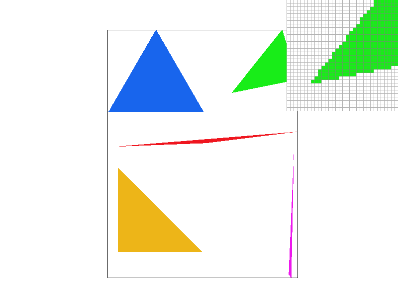
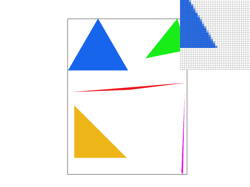
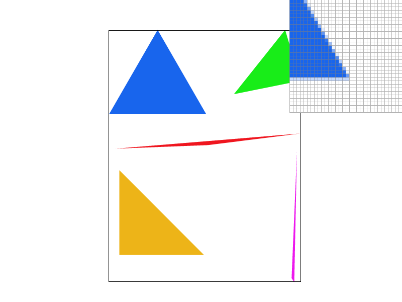
Supersampling allows for the sampling the image with a higher frequency where the square root of the sample rate determines the frequency of samples per pixel. By the nyquist criteria, the higher sampling rate allows for the representation of higher frequencies without aliasing that when downsampled to resolve into the framebuffer, contains information from these higher frequency samples. This is why supersampling is useful, as it allows for the representation of higher frequencies in our image without aliasing.

From the images, supersampling is demonstrated to be effective in sharpening edges and removing jaggies that we can observe in the single pixel sampling rate. The multi pixel sampling rates show different shades of blue that signify pixels that had corresponding samples that were inside the triangle according to the line equation. This method of rendering allows for this boundary to be more accurate to the floating point triangle boundary

Part 3: Transforms

The robot svg is trying to meditate after working tirelessly on this project :0. I'm glad the homogenous transformation matrices that were implemented helped change our protagonists positions.

Section II: Sampling

Part 4: Barycentric coordinates

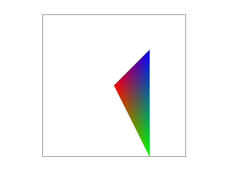
The barycentric coordinates are a way to represent the proportional distance from each of the vertices in a triangle as vector coordinates for any point in the triangle. Each (x,y) pair can be constructed as a linear combination of each of the different vertices of the triangle and the weights (alpha, beta, gamma) used in this combination can be used to continuously interpolate various things. The triangle below uses the barycentric coordinate weights to asign each point in the triangle weighted average of each of the vertex colors where the closer to the vertex you are, the larger the weight towards that certain color.

Part 5: "Pixel sampling" for texture mapping

Pixel sampling is a way of determining the values of pixels needed to render a textured polygon. As a reference for what colors need to appear spatially in the image, the texture map has its own set of coordinates in a coordinate space where each triangle vertex in the render space has a direct correlate for a vertex in the texture space.

For a specific sample coordinate (x,y), the texture coordinate is calculated using the barycentric weights and this coordinate (u, v) is used to sample the texture and assign the pixel a color value. The way this texure pixel is sampled can vary and the two methods that were implemented in this project were the nearest and bilinear pixel sampling methods.

The nearest pixel sampling method takes the (u, v) coordinate and finds the nearest pixel center coordinate and assigns that texture pixel value to the sample. Only the nearest pixel is used and no other information is interpolated to find pixel coordinates that are between pixel centers. The bilinear sampling method takes the surrounding 4 pixels and interpolates the linear distance between each pixel center. The ratio of the distance between the point and one of two vertices can be used as a weight to interpolate the color values as we did with the barymetric coordinates. The colors interpolated from the top and bottom pairs of points in x axis are then used as endpoints in a y axis interpolation.

The image shows a clear difference between the gradient of texture when using nearest sampling vs bilinear sampling. Due to the continuous interpolation of multiple points in the vicinity of the sample, bilinear sampling produces softer edges and less jagged pixel colors even when sampling only 1 sample per pixel. The biggest difference between the methods will probably arise when textures are applied with highly varying pixel colors. In the berkeley seal example, the blue and white edges are very sudden and due to the warping, the lines are not straight creating jaggies. The bilinear interpolation softens this boundary by sampling around the boundary and interpolating for samples that are on these edges contributing to a softer edge.

Part 6: "Level sampling" with mipmaps for texture mapping

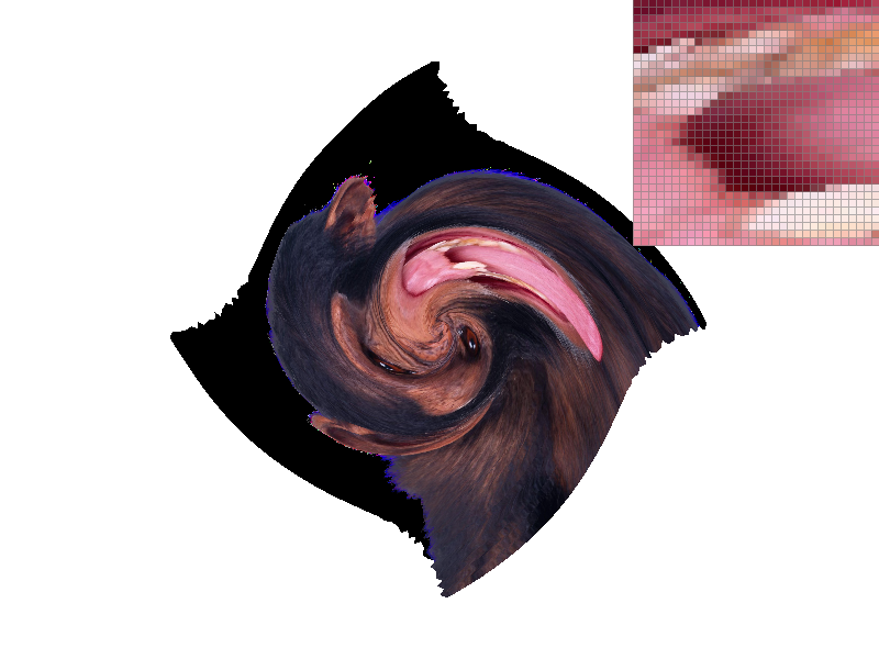
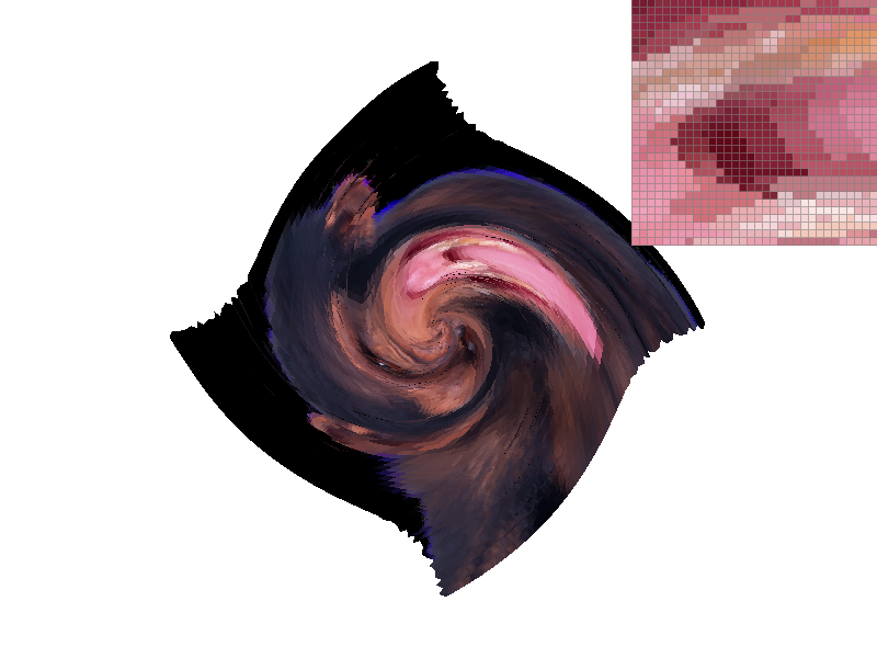
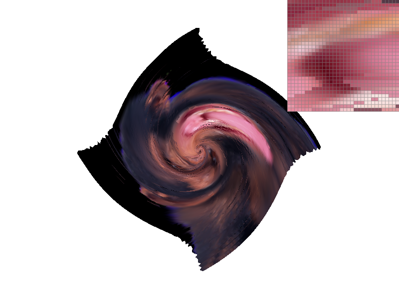
Level sampling allows for samples to be generated from lower frequency representations of textures based on how far the texture is and how translation in the pixel screen space maps to translation in the texture coordinate space. If translation in screen space coresponds to 2 units of travel in texture space, we can sample the texture colors from a texture that is half the width and half the size of the original image (level 1 mipmap). Since higher frequencies are removed from the new image we are sampling aliasing is reduced as these high frequencies can no longer act as lower frequency noise when undersampled. Since our pixel scaling is now 2 times our texture scaling we are essentially sampling at a lower spatial freqency on the texture image when we are zoomed out. The level combats the potential for aliasing. Once a continuous level value is calculated based on the magnitude of the texture differentials, either the closest level mipmap can be sampled or the color value from two levels can be interpolated linearly based on the continuous level value. This method is trilinear interpolation.

As one can notice from the images, the level creates a downsampled texture that is sampled and overlayed on the polygon based on the object translations. Using the nearest level therefore results in a smoother image especially since we are zoomed out in these images. The antialiasing is especially noticable when comparing the left images since we can see artifacts on the border of the monkey and the background while using the nearest level these edges are smoothed out. Level sampling therefore provides some degree of antialiasing power. In addition, as we've seen previously the bi-linear texture sampling further increases sampling rate to combat aliasing. Observe the whites of the monkey's eyes as the antialiasing increases.

The tradeoffs for the techniques come with memory and speed respectively. In the implementation that I worked on, a set of texture mip levels were stored for a texture that contained downsampled versions of the original texture. This is extra memory overhead when not using level sampling. However, due to the nature of reducing the dimensions of the images by half each time, storing mip maps only takes one third more memory than if we only stored the original texture. Essentially, the mip maps fit in one extra channel of the original texture making this relatively space efficent. Speed is comprimised noticably when using bilinear sampling since now each sample requires accessing 4 texture pixel values and running 3 linear interpolations. This is opposed to only accessing one texture pixel using nearest sampling. Generally, level sampling seems to provide antialiasing support when zoomed out of an image and the bilinear filter provides smoothing when zoomed in close.

gundralaa.github.io/cs184p1.html

Writeup Website