Ray Tracer
https://gundralaa.github.io/2023/03/20/cs184-ray-tracer.html
CS184 Project 3-1
Abhinav Gundrala
Overview
The ray tracer project for CS 184 Computer Graphics required the implementation of key algorithms used in calculating realistic lighting in scenes by tracing rays. Each part of the project deals with tracing and sampling rays of light through a scene to ultimately calculate the color intensity of a specific pixel on the grid. Objects in the scene are mathematically represented as primitives and ray interaction with these objects is used to simulate obstruction, shadows, reflection and other interesting lighting phenomena. Following are descriptions of key algorithms and resultant images from the tracer.
Rays and Primitives
Part 1
Ray Generation
Rays are characterized using two fields. Each ray has an origin point in a space and a unit normalized vector denoting the direction. We trace light rays from a fixed camera point through a sensor plane of a fixed width and height. Each position on the image coresponds with a specific position on the sensor plane in the world coordinates. To calulate the value of a single pixel on the sensor plane, a set of rays are sampled that pass through the pixel on the sensor plane. Each of these generated rays are traced through the scene to calculate the global illumination vector, a 3D color vector, for each pixel.
Primitive Intersection
Primitives are objects in the scene that light rays interact with to render a scene. Primitive intersection deals with calulating if and where on a surface a particular generated ray intersects. This information is important for lighting effects since the angle at which the light ray is incident with respect to the primitive surface normal determines properties of the brightness of the light and creates the effect of shading. Images below help illustrate where calculating the normal at a surface ray intersection is important due to the realistic shading effects.
Triangle Intersection Algorithm
To calculate a triangle intersection, I used the Moller Trumbore Algorithm to efficently caluclate the barycentric coeffients of the point of intersection in the triangle and the t value for tracing the ray. Calculating a specific point on a ray becomes [P = Ot + D] where [t] must be positive for an intersection to have occured. The algorithm allows for both the checking if the ray intersects the triangle plane and if the hit point is within the bounds of the triangle using the barycentric coordinates.
Using the matrix formulation of the equation. Each of t, b1 and b2 are calculated using the calculated vectors. First the algorithm checks if the the ray direction is parallel to the triangle by taking the cross product of the ray direction and each edge of the triangle originating from a single point p0. The these cross products can be used to calculate first if the ray is parallel to the triangle. Then the algorithm checks if the sum of b1 and b2 are within the range of [0.0, 1.0]. Finally the t value is calculated and if it is within the range of possible intersection, a intersection is returned. When an intersection occurs the maximum range for the next intersection is shortened to the current hit point. This is to ignore ray intersections of a primitive that is behind another.
  double eps = 0.0000001;
  double a, b_1, b_2, t;
  Vector3D e1, e2, s, s1, s2;

  e1 = p2 - p1;
  e2 = p3 - p1;
  s1 = cross(r.d, e2);
  a = dot(e1, s1);
  // check ray is parallel
  if (a > -eps && a < eps)
    return false;

  s = r.o - p1;
  b_1 = (1/a) * dot(s, s1);
  if (b_1 < 0.0 || b_1 > 1.0)
    return false;

  s2 = cross(s, e1);
  b_2 = (1/a) * dot(r.d, s2);
  if (b_2 < 0 || b_1 + b_2 > 1.0)
    return false;

  t = (1/a) * dot(e2, s2);
  if (t > r.min_t && t < r.max_t)
  {
    r.max_t = t;
    return true;
  }
  return false;
Image Examples
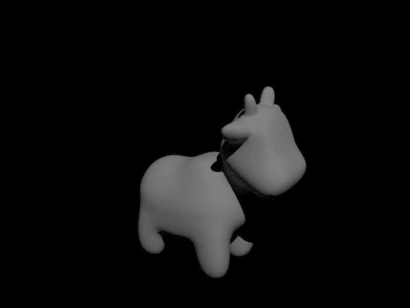
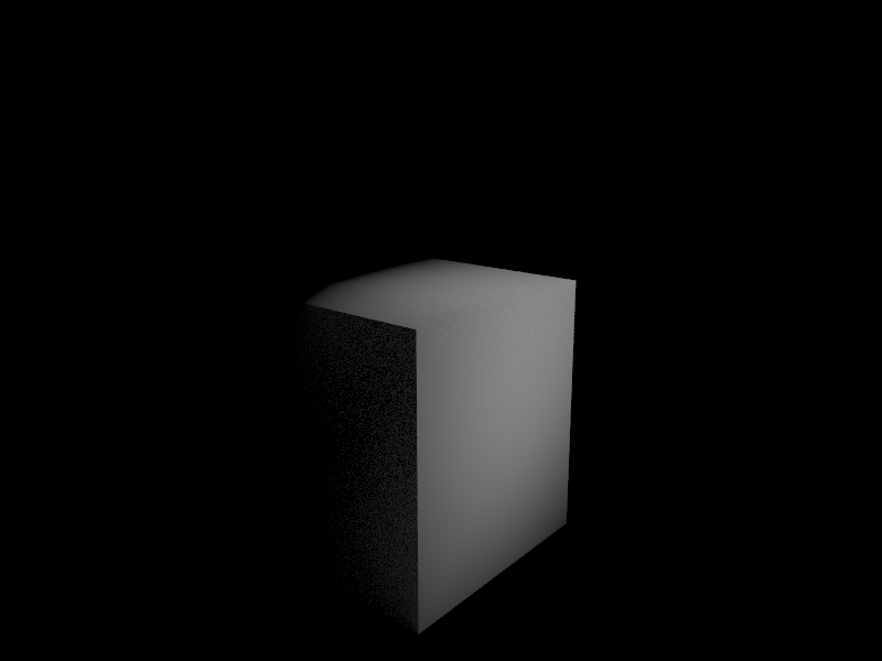
Below are some examples of images that were normal shaded using the barycentric normal calulation using the hit point. Due to lamberts cosine law, the recieved irradiance at a surface is directly proportional to the dot product between the surface normal and the incoming light ray. These images demonstrate the shading due to this principle.
Cow
Cube
Bounded Volume Hierarchy
Part 2
BVH Construction
To accelerate ray to primitive intersection calculations, the BVH construction algorithm constructs a heirarchical tree of bounding boxes that hold groups of primitives in leaf nodes of the tree. Each non-leaf node defines a bounding box that encapsulates all primitives underneath the node in the tree. Traversing the BVH allows reducing the number of primitives to search when checking ray intersection in the scene. Instead of iterating through all volumes, we can check intersection with each bounding box in the tree and traverse the child that contains an intersection.
When constructing the tree, at each call of the recursion a start and end pointer are provided to define the set of primitives to be split at that specific level. First an axis for the split is chosen by checking the axis with the maximum range for centroids in the node. This heuristic is chosen to maximize the distance between centroids in the children. After the axis is chosen, the subset of the primitive list is sorted by centroid in ascending order. The splitting point is chosen as the midpoint of the centroid range and the list of primitives is iterated through till the centroid axis value for a primitive exceeds the splitting point. The splitting methods is then recursively called using this new midpoint as the end pointer for the left child and the start pointer for the right child.
The code below represents the in-place sorting operation and determining the split point iterator for recursion for one axis where all axis are included in a switchstatement.
  std::sort(start, end,
    [](Primitive* a, Primitive* b) {
      return a->get_bbox().centroid().x < b->get_bbox().centroid().x;
    }
  );
  mid = end;
  for (auto p = start; p != end; p++) {
                            BBox bb = (*p)->get_bbox();
    Vector3D c = bb.centroid();
    // set mid as middle
    if (c.x > ((maxes[0] + mins[0]) / 2)) {
      mid = p;
      break;
    }
  }
Images
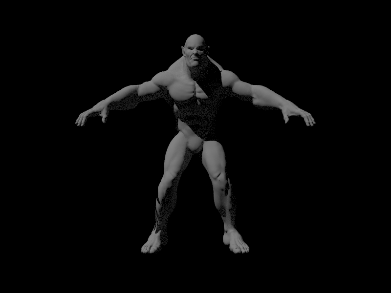
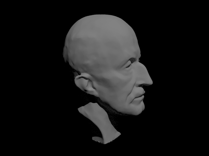
The images here contain hundreds of thousands of primitives that iterating through all of them to find ray intersections would be exponentially time consuming. The BVH reduces the complexity of the search and drastically improves the render.
Beast
Max Planck
Rendering Time Analysis
Rendering the beast was almost impossible without a bvh traversal. Due to this operation taking too long the cow was chosen to render instead. Without the BVH optimizations before rendering, the cow took approximately 813 seconds to render locally with features up to part 2 with normal shading. When optimized the new render took 156 seconds.
Direct Lighting
Part 3
Ray Tracing Implementation
The ray tracer follows rays originating from the camera that pass through specific pixels in the sensor plane. Each ray is then checked for intersection in the scene and the point of intersection defines the light that travels across the ray back to the pixel. To estimate the direct light at the hit point of a ray, rays in a hemisphere with an origin at the hit point are sampled. The sampled rays are traced to check if an intersection with a light is found. If this is the case, the emission from the light is weighted by the angle of incidence and the surface bsdf which in this case is a diffuse surface. The sampling follows a monte carlo scheme to estimate the reflection integral. The sum of sample outgoing radiance is divided by the number of samples and each sample is weighted by the pdf of the sampler.
To reduce noise in the integral calculation due to hemisphere sampling, importance sampling is used to only samples sources of light and rays that originate from lights and end at the hit point. Each light source is iterated through and a set of rays are sampled from each light source based on the type of light. For point lights there is only one ray sample possible therefore only one sample is taken. As before, the outgoing radiance is calculated using the reflection equation and the estimator is weighted by the pdf and the number of samples for each light.
Images
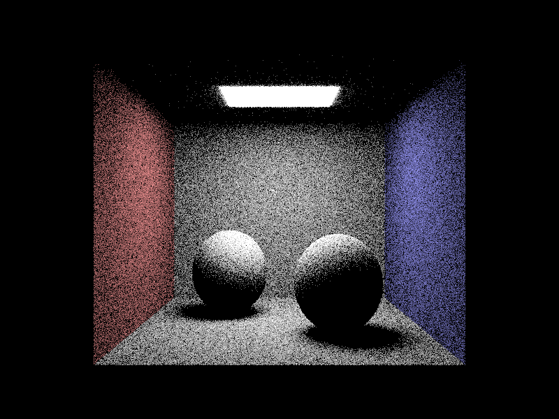
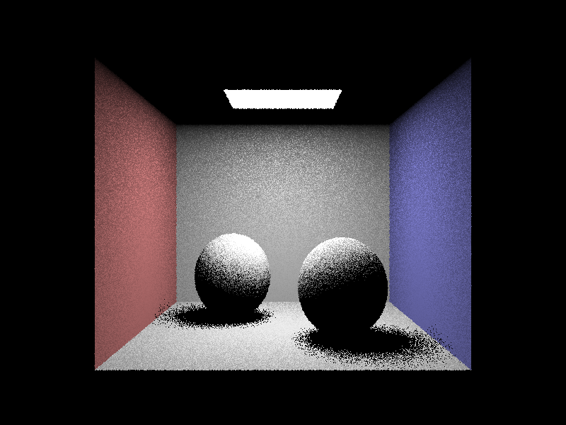
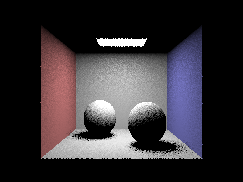
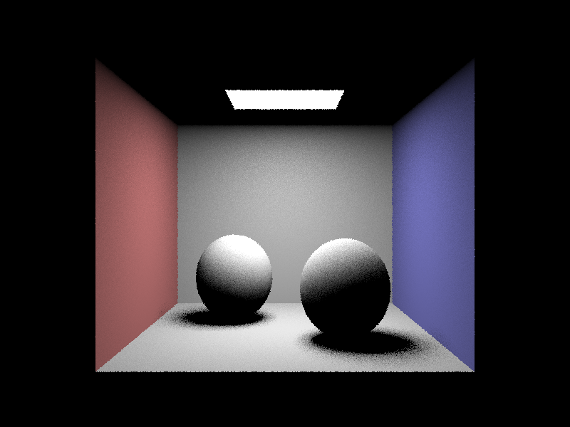
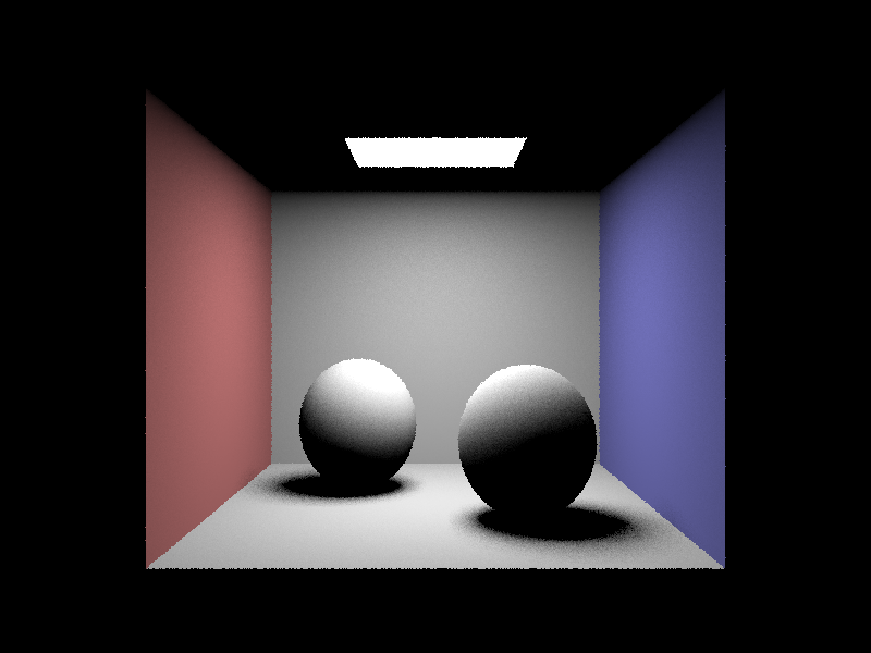
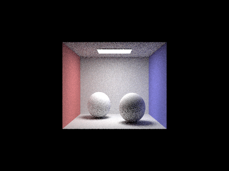
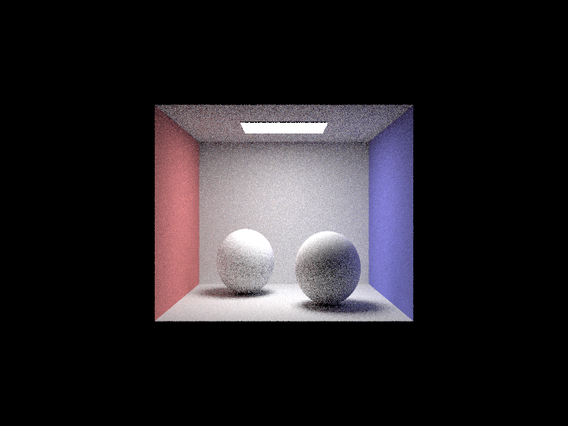
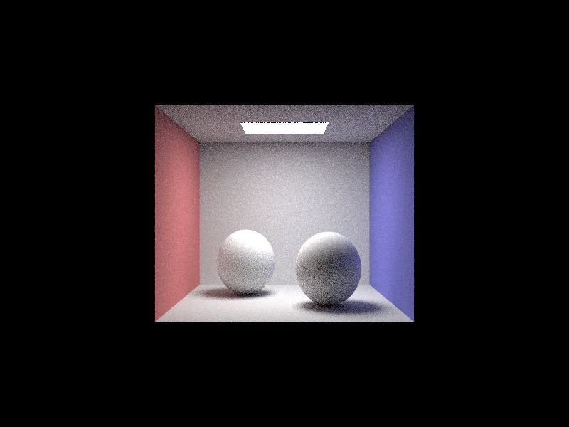
For this specific scene here are renders that use the different direct lighting sampling techniques. For the images rendered using importance sampling on the lights in the scene, the number of light rays sampled for each area light was varied. All pixels were sampled with one ray.
Uniform Hemisphere Sampling
Light Rays 1
Light Rays 4
Light Rays 16
Light Rays 64
Comparing Sampling Methods
As observable from the images above, uniform hemisphere sampling produces a large amount of noise due to the integral being estimated using rays that have very little impact on the irradiance arriving at a hit point. Any ray that does not intersect a light when calulating direct lighting does not contain useful information yet. There is significantly less noise when sampling lights and increasing the number of light rays used to sample each area light reduces noise further.
Indirect Lighting
Part 4
Ray Tracing Implementation
Scenes become much richer when more than one bounce of light is calculated and rendered. With direct lighting only ray paths originating from light sources that hit objects in the scene to reflect on to the sensor plane are used in calculating the radiance along a pixel. However, light from other objects in the scene can reflect and also intersect the same hit point altering the radiance along the camera ray. Adding indirect lighting allows for a more detailed and realistic render.
The indirect lighting algorithm recursively calculates the radiance of a ray at an intersection by adding the direct lighting contribution at each intersection and recursively calling the indirect lighting method on a number of sampled rays from the hit point hemisphere. The reflectance equation is applied again to calcuate the outgoing radiance. Recursion for ray tracing stops when either the recursion depth hits some max value or a russian roulette termination condition is reached. The probablity of termination was set to p=0.4.
Images
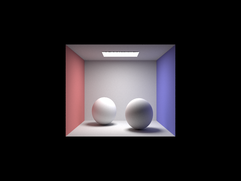
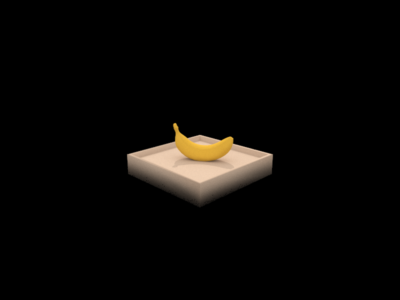
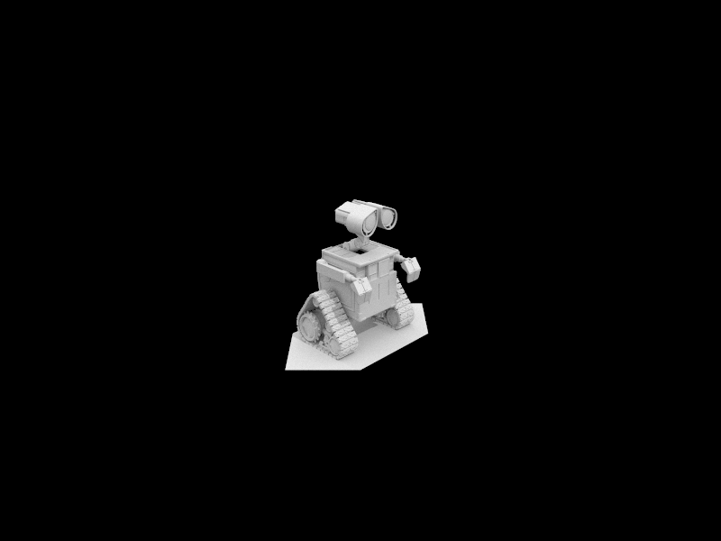
Here are some very gorgeous renders that used both direct and indirect illumination in the scene. These are high quality renders that use 1024 samples for each pixel.
spheres; will see them again
this is the most beautiful bannana I have seen
wall-e took years to render
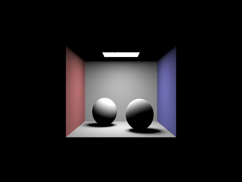
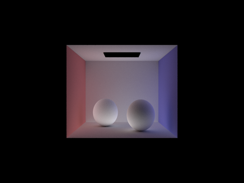
The renders below illustrate the components of a scene that depend on direct and indirect illumination only. Direct illumination includes one and zero bounce light rays while indirect illumination is for light contributed from any non light source.
Direct Lighting
Indirect Lighting
Bunny Renders
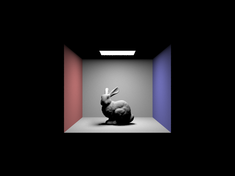
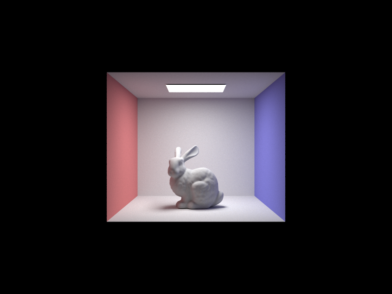
Here are a set of renders that place a bunny model in cornell box with one area light at the top. Each view has a different max ray depth set for indirect lighting calculations that limits the number of bounces one ray can have before termination.
Max Ray Depth 0
Max Ray Depth 1
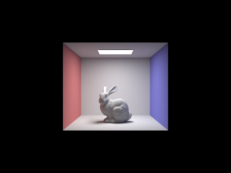
Max Ray Depth 3
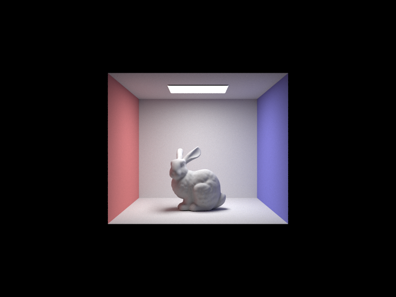
Max Ray Depth 100
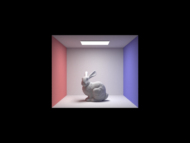
Overall, there seem to be diminishing returns in tracing rays to this depth in such a simple scene. Maybe with more complex light interactions a depth of a 100 would be reasonable.
Pixel Sample Rates
The renders below compare rendering the sphere scene using different pixel sample rates. Increasing the sampling rate should theoretically reduce noise in the scene but also trace a larger number of ray in the scene to capture larger range of light interactions.
Sample Rate 1

Sample Rate 2
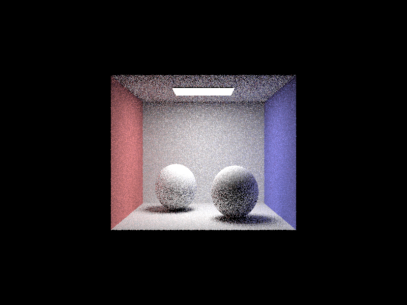
Sample Rate 4
Sample Rate 8
Sample Rate 16
Sample Rate 64

Sample Rate 1024

Adaptive Sampling
Part 5
Sampling Implementation
Some pixels don’t need to be sampled as vigorously as other pixels due to a low variance in samples. These pixels converge quickly and don’t require a large number of samples. Adaptive sampling calculates the variance of samples as the pixel is sampled to terminate early when the estimated radiance is within the 95% confidence interval. For each sample, the sum and squared sum are calcuated and after a sample batch number of samples the mean and variance of samples so far is calculated. When the confidence exceeds some threshold, the loop is broken and the number of samples is recorded to weight the sample sum.
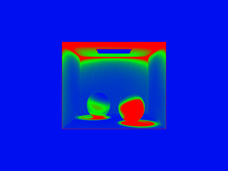
Images
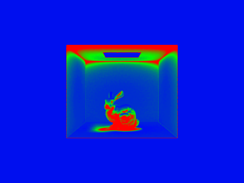
Each scene is rendered with a maximum of 2048 samples per pixel but using adaptive sampling, some pixels are sampled at high sampling rates and some lower. Blue reprepresents a low number of samples meaning the illuminance converge early and red represents a high number of samples.
Bunny Render
Bunny Render Rate
Sphere Render

Sphere Render Rate